SliceViewer Testing

Introduction

The Sliceviewer in Workbench has the joint functionality of the SpectrumViewer and SliceViewer from MantidPlot. So while the advanced use cases for multi-dimensional diffraction data are important to test, it is also worth checking more basic uses, for example opening a Workspace2D and examining the subplots and dynamic cursor data.

See here for a brief overview of the Sliceviewer.

Basic Usage

MatrixWorkspace

Do the following tests with an EventWorkspace (e.g. CNCS_7860_event.nxs) and a Workspace2D (e.g. MAR11060.raw) from the TrainingCourseData.

1. Load the workspace and open in sliceviewer (right-click on the workspace in the ADS > Show Slice Viewer).

2. Confirm that for MatrixWorkspaces the Peak overlay, Nonorthogonal view and Non-axis aligned cutting tool buttons should be disabled (greyed out).

3. Check the other toolbar buttons.

   1. Pan and Zoom (use mouse scroll and magnifying glass tool) and Home

      • As you zoom check the color scale changes if autoscale checked in checkbox below colorbar).

   2. Toggle grid lines on/off

   3. Enable line plots

      • Confirm the curves update with the cursor position correctly

   4. Export cuts to workspaces in ADS using keys x, y, c

      • This should produce workspaces in the ADS with suffix _cut_x and _cut_y

      • Plot these in workbench check they agree with sliceviewer plots

   5. Disable line plots and Enable ROI tool

      

      • The line plot button should be automatically enabled

   6. Draw, move and resize the rectangle

      • Move it off the axes (it should just clip itself to be contained within the axes).

      • Export the cuts with keys x, y, c

      • In addition the ROI can be exported by pressing r

        • This should produce another workspace with suffix _roi

        • Open it in sliceviewer and check the data and limits agree with the ROI drawn.

   7. Disable the ROI tool

      • The line plot tool should remain enabled.

4. Try saving the figure (with and without ROI/lineplots).

5. Test the colorbar and colorscale

   1. Change normalisation

      • The color limits should only change if autoscale is enabled.

   2. Change the scale type to e.g. Log

      • In Log scale bins with 0 counts should appear white

      • When you zoom in to a region comprising only of bins with 0 counts it will set the color axis limits to (0.1,1) and force the scale to be linear

      • Zoom in to a region outside the extent of the data, check the Log colorscale option is disabled.

   3. Change colormap

   4. Reverse colormap

   5. Change auto-scale option from default Min/Max to another e.g. 3-sigma

6. Test transposing axes: click the Y button to the right of the Time-of-flight label (top left corner) - the image should be transposed and the axes labels updated.

7. Test the Cursor Information Widget (table at top of sliceviewer window with TOF, spectrum, DetID etc.)

   1. Confirm it tracks with the cursor when Track Cursor is checked

   2. Uncheck the track cursor and confirm it updates when the cursor is clicked.

   3. Transpose the axes (as in step 6) and confirm the cursor position displayed is still correct.

8. Resize the sliceviewer window, check the widgets, buttons etc. are still visible and clear for reasonable aspect ratios.

MD Workspaces

MD workspaces hold multi-dimensional data (typically 2-4D) and come in two forms: MDEventWorkspace, MDHistoWorkspace. In terms of sliceviewer functionality, the key difference is that MDHistoWorkspace have binned the events onto a regular grid and cannot be dynamically rebinned unless the original MDWorkspace (that holds the events) exists in the ADS (and the MDHistoWorkspace has not been altered by a binary operation e.g. MinusMD).

MDWorkspace (with events)

1. Create a 3D and 4D MDWorkspaces with some data - repeat the following tests with both md_4D and md_3D. Note this will throw a warning relating to the SlicingAlgorithm.

from mantid.simpleapi import *

md_4D = CreateMDWorkspace(Dimensions=4, Extents=[0,2,-1,1,-1.5,1.5,-0.25,0.25], Names="H,K,L,E", Frames='HKL,HKL,HKL,General Frame',Units='r.l.u.,r.l.u.,r.l.u.,meV')
FakeMDEventData(InputWorkspace=md_4D, UniformParams='5e5') # 4D data
FakeMDEventData(InputWorkspace=md_4D, UniformParams='1e5,0.5,1.5,-0.5,0.5,-0.75,0.75,-0.1,0.1') # 4D data

# Add a non-orthogonal UB
expt_info = CreateSampleWorkspace()
md_4D.addExperimentInfo(expt_info)
SetUB(Workspace='md_4D', c=2, gamma=120)

# make a 3D MDEvent workspace by integrating over all E
md_3D = SliceMD(InputWorkspace='md_4D', AlignedDim0='H,0,2,100', AlignedDim1='K,-1,1,100', AlignedDim2='L,-1.5,1.5,100')

# Create a peaks workspace and fake data in 3D MD
CreatePeaksWorkspace(InstrumentWorkspace='md_3D', NumberOfPeaks=0, OutputWorkspace='peaks')
CopySample(InputWorkspace='md_3D', OutputWorkspace='peaks', CopyName=False, CopyMaterial=False, CopyEnvironment=False, CopyShape=False)
AddPeakHKL(Workspace='peaks', HKL='1,0,1')
AddPeakHKL(Workspace='peaks', HKL='1,0,0')

2. Test the toolbar buttons pan, zoom, line plots, ROI as in step 3 of the MatrixWorkspace instructions.

   • This workspace should be dynamically rebinned - i.e. the number of bins within the view limits along each axis should be preserved when zooming.

   • The cursor info table should also display the HKL of the cursor

3. Change the number of bins along one of the viewing axes (easier to pick a small number e.g. 2)

4. Change the integration-width/slice-thickness (spinbox to the left of the word thick) along the non-viewed axes.

   • Increasing the width should improve the stats on the uniform background and the color limit should increase (event counts are summed not averaged).

5. Change the slicepoint along one of the non-viewed axes

   1. Confirm the slider moves when the spinbox value is updated.

   2. Confirm moving the slider updates the spinbox.

   3. Check the slicepoint is updated in the cursor info table.

Test the Nonorthogonal view

1. Click the nonorthogonal view button in the toolbar

   • This should disable ROI and lineplot buttons in the toolbar

   • This should automatically turn on gridlines

   • When H and K are the viewing axes the gridlines should not be perpendicular to each other

   • The features in the data should align with the grid lines

2. Zoom and pan

   • Confirm the autoscaling of the colorbar works in non-orthogonal view

3. Change one of the viewing axes to be L (e.g. click X button next to L in top left of window)

   • Gridlines should now appear to be orthogonal

4. For md_4D only change one of the viewing axes to be E (e.g. click Y button next to E in top left of window)

   • Nonorthogonal view should be disabled (only enabled for momentum axes)

   • Line plots and ROI should be enabled

   • Change the viewing axis presently selected as E to be a momentum axis (e.g. H)

     • The nonorthogonal view should be automatically re-enabled.

Test the Peak Overlay

1. Click to peak overlay button in the toolbar

2. Check the Overlay? box next to peaks

   • This should open a table (peak viewer) on the RHS of the sliceviewer window - it should have two rows corresponding to peaks at HKL = (1,0,1) and (1,0,0).

3. Double click a row

   • It should change the slicepoint along the integrated momentum axis and zoom into the peak - e.g. in (X,Y) = (H,K) then the slicepoint along L will be set to 1 and there will be a cross at (0,0).

   • Note for md_4D a peak will not be plotted if a non-Q axis is viewed, if both axes are Q-dimensions then the cross should be plotted at all E (obviously a Bragg peak will only be on the elastic line but the peak object has no elastic/inelastic logic and the sliceviewer only knows that E is not a momentum axis, it could be temperature etc.).

4. Click Add Peaks in the Peak Actions section at the top of the peak viewer (note for 4D workspaces the peak overlay won’t work for non_Q dimensions).

5. Click somewhere in the colorfill plot

   • Confirm a peak has been added to the table at the position you clicked

   • Note that peaks need to have H > 0 to be valid due to the assumed beam direction (otherwise you will get an error in the log ValueError: Peak::setQLabFrame(): Wavelength found was negative)

6. Click Remove Peaks

7. Click on the cross corresponding to the peak you just added

   • Confirm the correct row has been removed from the table

   • The cross should be removed from the plot

8. Repeat the above steps 1-7 in non-orthogonal view.

9. Check the Concise View checkbox above one of the peak tables on the right hand side - this should hide some columns.

MDHistoWorkspace

1. Make a 3D MDHistoWorkspace

md_3D_histo = BinMD(InputWorkspace='md_4D', AlignedDim0='H,-2,2,100', AlignedDim1='K,-1,1,100', AlignedDim2='L,-1.5,1.5,100')

2. Open md_3D_histo in sliceviewer it should not support dynamic rebinning (can’t change number of bins).

3. Test the toolbar buttons pan, zoom, line plots, ROI as in step 3 of the MatrixWorkspace instructions.

4. Test changing/swapping viewing axes

5. Test the Nonorthogonal view as above

6. Open md_4D_svrebinned in sliceviewer (should be in the ADS after preceding tests).

   • It should support dynamic rebinning (i.e. will be able to change number of bins along each axis).

7. With md_4D_svrebinned open in the sliceviewer, delete md_4D in the ADS.

   • It should close sliceviewer because the support for dynamic rebinning has changed

8. Open md_4D_svrebinned in sliceviewer again

   • It should no longer support dynamic rebinning

   • Confirm transposing axes works

CutViewer Tool

1. Check the Non-axis aligned cutting tool button is only enabled for 3D MD workspaces where all dimensions are Q by opening the following workspaces in sliceviewer. It should only be enabled for the ws_3D and ws_3D_QLab workspaces (see comment for details) - the first 3 column headers for the vectors should be a*,b*,c* and Qx,Qy,Qz for the two workspaces respectively.

Load(Filename='CNCS_7860_event.nxs', OutputWorkspace='CNCS_7860_event')  # disabled (MatrixWorkspace)

ws_2D = CreateMDWorkspace(Dimensions='2', Extents='-5,5,-4,4', Names='H,K',
                          Units='r.l.u.,r.l.u.', Frames='HKL,HKL',
                          SplitInto='2', SplitThreshold='50')  #  disabled (2D MD)

ws_3D = CreateMDWorkspace(Dimensions='3', Extents='-5,5,-4,4,-3,3',
                          Names='H,K,L', Units='r.l.u.,r.l.u.,r.l.u.',
                          Frames='HKL,HKL,HKL', SplitInto='2', SplitThreshold='50')  # enabled!

ws_3D_nonQdim = CreateMDWorkspace(Dimensions=3, Extents=[-1, 1, -1, 1, -1, 1],
                          Names="E,H,K", Frames='General Frame,HKL,HKL',
                          Units='meV,r.l.u.,r.l.u.')  # disabled (3D but 1 non-Q)

ws_4D = CreateMDWorkspace(Dimensions=4, Extents=[-1, 1, -1, 1, -1, 1, -1, 1],
                          Names="E,H,K,L", Frames='General Frame,HKL,HKL,HKL',
                          Units='meV,r.l.u.,r.l.u.,r.l.u.')  # disabled (4D - one non-Q)

ws_3D_QLab = CreateMDWorkspace(Dimensions='3', Extents='-5,5,-4,4,-3,3',
                               Names='Q_lab_x,Q_lab_y,Q_lab_z', Units='U,U,U',
                               Frames='QLab,QLab,QLab', SplitInto='2', SplitThreshold='50')  # enabled!

2. Close any sliceviewer windows and clear the workspaces in the ADS

3. Run the following and open ws in sliceviewer.

ws = CreateMDWorkspace(Dimensions='3', Extents='-5,5,-4,4,-3,3',
                          Names='H,K,L', Units='r.l.u.,r.l.u.,r.l.u.',
                          Frames='HKL,HKL,HKL', SplitInto='2', SplitThreshold='50')
expt_info = CreateSampleWorkspace()
SetUB(expt_info, 1,1,2,90,90,120)
ws.addExperimentInfo(expt_info)
# make some fake data
FakeMDEventData(ws, UniformParams='1e5', PeakParams='1e+05,0,0,1,0.3', RandomSeed='3873875')

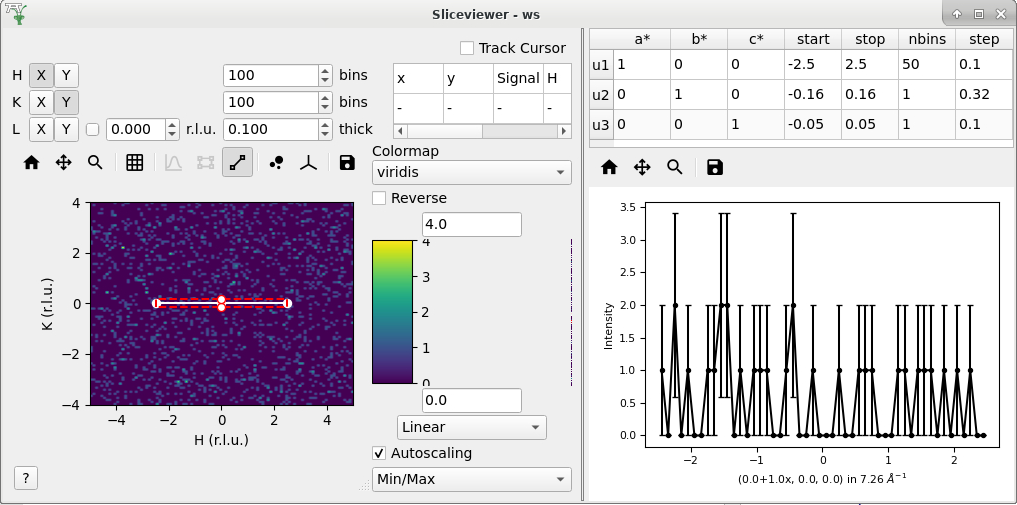
4. Open the cut tool and check that:

   • Disabled ROI tool

   • Disabled line plots

   • Sliceviewer should look like

6. Check that transposing the axes (X <-> Y) will swap the u1 and u2 vectors in the table

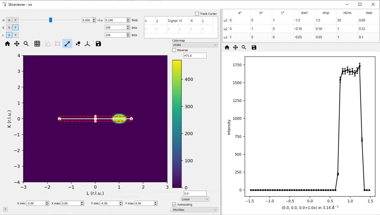
7. Set the axes to (X,Y) = (L, K) - check u1 = [0,0,1] and u2 = [0,1,0]

8. Change the slice point of H to be 0 - it should look like this

9. In the table double the step along u1 (i.e. set step to 0.12) - this should change nbins = 25 along u1

10. Set the nbins = 50 along u1 - the step should go back to it’s original value (0.06)

11. Set the stop for u1 to 0 and check that

    • step size = 0.03

    • the cut representation line on the colorfill plot has the correct start/stop

    • the 1D plot in the cut viewer pane has the correct axes limits

12. Set step of u1 to be 2 (i.e. greater than the extent of the cut) - this should set nbins=1 and step = 1.5 and put the cut along u2 with nbins = 50.

13. Transpose the axes so now (X,Y) = (K,L) - the cut should have 50 bins along K (default value)

14. Change the nbins of u2 to 50 (it should set nbins=1 for u1 and change the step=4). Check the white line of the cut representation on the colorfill plot is now vertical.

15. Try to change the a* column of the u1 to 1 (this would take u1 out of the plane of the slice, i.e. not orthogonal to u3) - it should reset to 0 - i.e. u1 = [0,1,0].

16. Click and hold down on one of the red markers with white face on the colorfill plot and drag, release at ~K=1.

    • This should reset the vectors in the table such that the cut is along u1 = [0,0,1] - i.e. u1 and u2 are swapped

    • The thickness along u2 should be adjusted to ~2

17. Set the step of u2 = 2 in the table, check that it sets (start,stop) = (-1,1)

18. Drag the top white marker of the cut representation up to L~2

    • u1 ~ [0,0,1] and u2 ~ [0,1,0]

    • There should be a peak in the 1D plot at x~1

19. For u1 set b*=0 and c* = -1 and start=-2 - check that u2 = [0,-1,0] and there is a peak at x~-1

20. To change the centre of the cut move the central white marker of the cut representation to (K,L) ~ (2,0),

    • The entire cut representation should move

    • The axes label of the 1D plot should be similar to (0.0, 2.0,0.0-1.0x) in 3.14 Ang^-1

    • There should be no peak on the 1D plot

21. Increase the thickness by dragging the left red marker of the cut representation to encompass the peak in the data - check the peak appears in the 1D plot at the right thickness.

22. Play around with the direction of the cut by dragging the white markers at the end points of the white line - the vectors u1 and u3 should be orthogonal unit vectors.

23. Reset the cut by transposing the axes so (X,Y) = (L,K)

24. Double the slice thickness along H from 0.1 -> 0.2 (the counts of the peak in the 1D plot should double from ~2000 -> ~4000)

25. Change c* of u1 from 1 -> -1

    • The peak in the 1D plot should move from x= 1 -> -1

    • Check u2 = [0,-1,0]

26. Turn on non-orthogonal view and play around with the cut tool representation

    • Check that the table values are updated correctly (use the HKL in the cursor info table to help determine this)

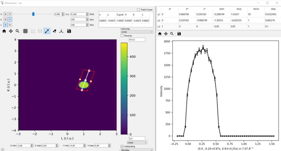
27. Produce a non-axis aligned cut where the peak is not in the center of the x-range. Take the x-value at the peak maximum and plug it into the axis label - it should produce the HKL of the peak (0,0,1).

Specific Tests

1. Representation of integrated peaks

1. Run the code below to generate fake data and integrate peaks in the 3D MDWorkspace md_3D from MDWorkspace (with events)

# Fake data in 3D MD and integrate
FakeMDEventData(md_3D, EllipsoidParams='1e4,1,0,1,1,0,0,0,1,0,0,0,1,0.005,0.005,0.015,0', RandomSeed='3873875') # ellipsoid
FakeMDEventData(md_3D, EllipsoidParams='1e4,1,0,0,1,0,0,0,1,0,0,0,1,0.005,0.005,0.005,0', RandomSeed='3873875')  # spherical
IntegratePeaksMD(InputWorkspace='md_3D', PeakRadius='0.25', BackgroundInnerRadius='0.25', BackgroundOuterRadius='0.32', PeaksWorkspace='peaks', OutputWorkspace='peaks_int_ellip', IntegrateIfOnEdge=False, Ellipsoid=True, UseOnePercentBackgroundCorrection=False)
IntegratePeaksMD(InputWorkspace='md_3D', PeakRadius='0.25', BackgroundInnerRadius='0.25', BackgroundOuterRadius='0.32', PeaksWorkspace='peaks', OutputWorkspace='peaks_int_sphere', IntegrateIfOnEdge=False, Ellipsoid=False, UseOnePercentBackgroundCorrection=False)
IntegratePeaksMD(InputWorkspace='md_3D', PeakRadius='0.25', BackgroundInnerRadius='0', BackgroundOuterRadius='0', PeaksWorkspace='peaks', OutputWorkspace='peaks_int_no_bg', IntegrateIfOnEdge=False, Ellipsoid=False, UseOnePercentBackgroundCorrection=False)
# IntegratePeaksMD will throw an error
#   Error in execution of algorithm MaskBTP:...
# This is because the simulated ws don't have a real instrument but the integration will be executed

2. Open md_3D in sliceviewer

3. Click the peak overlay button in the toolbar

4. Overlay peaks_int_ellip and peaks_int_sphere

5. Click the first row in the first table

   • It should zoom to a peak.

   • There should be an ellipse and a circle drawn with dashed lines with different colors (the color should match the color of the workspace name in the peak viewer table).

   • There should be a transparent shell indicating the background for each peak.

   • The ellipse should be smaller than the circle.

6. Alter the slice point by moving the slider along the integrated dimension

   • The circle and ellipse should shrink

   • There should be no gap between the background shell and the dashed line.

7. Click on the second row on the second table.

   • It should zoom in on a different peak.

   • The ellipse and circle should be very similar (not quite same as the covariance matrix was evaluated numerically for randomly generated data).

8. Click the nonorthogonal view button

9. The ellipse and circle should still agree with each other and the shape of the generated data.

10. Click the Peak overlay button in the toolbar

11. Overlay the peaks_int_no_bg workspace and remove peaks_int_sphere

12. Zoom in on a peak (click a row in the table)

    • There should be a dashed line but no background shell for peaks in peaks_int_no_bg

Keep the three peak workspaces overlain for the next test.

2. ADS observer for peak overlay

1. Rename peaks_int_ellip in the ADS to e.g. peaks_int_ellipse

   1. Confirm the name changes in the peak viewer table

   2. Click on a peak, the ellipse should still be drawn on the colofill plot

2. Remove a row from peaks_int_no_bg table (open table from ADS > Right-click on a row > Delete)

   1. Confirm the correct row is removed from the corresponding row in the peak viewer table

   2. Click on the peak in the peaks_int_ellipse table that has been removed from peaks_int_no_bg

      • Only the ellipse should be plotted.

3. Delete peaks_int_no_bg from the ADS

   • The table should be removed from the peaks viewer

   • Confirm the Peak actions combo box is updated to only contain peaks_int_ellipse

4. Delete peaks_int_ellipse from the ADS

   • The peak overlay should be turned off and the table hidden

3. ADS observer for workspace

With md_3D open in sliceviewer

1. Rename md_3D to e.g. md_3Dim

   • The workspace name in the title of the sliceviewer window should have updated

   • Zoom to check dynamic rebinning still works

2. Ensure colorbar autoscale is checked.

3. Take a note of the colorbar limits and execute this command in the ipython terminal

   mtd['md_3Dim'] *= 2
   

   • The colorbar max should be doubled.

   • Zoom to check dynamic rebinning still works

4. Clone the workspace for future tests

CloneWorkspace(InputWorkspace='md_3Dim', OutputWorkspace='md_3D')

5. Delete md_3Dim in the ADS

   • The sliceviewer window should close

4. ADS observer for support for nonorthogonal view

1. Open md_3D in sliceviewer

2. Run ClearUB algorithm on md_3D

   • Sliceviewer window should close with message Closing Sliceviewer as the underlying workspace was changed: The property supports_nonorthogonal_axes is different on the new workspace.

5. Check BinMD called with NormalizeBasisVectors=False for HKL data

1. Create a workspace with peaks at integer HKL and take a non axis-aligned cut

ws = CreateMDWorkspace(Dimensions='3', Extents='-3,3,-3,3,-3,3',
                       Names='H,K,L', Units='r.l.u.,r.l.u.,r.l.u.',
                       Frames='HKL,HKL,HKL',
                       SplitInto='2', SplitThreshold='10')

# add fake Bragg peaks for primitive lattice in data
for h in range(-3,4):
    for k in range(-3,4):
        for l in range(-3,4):
            hkl = ",".join([str(x) for x in [h,k,l]])
            FakeMDEventData(ws, PeakParams='1e+02,' + hkl + ',0.02', RandomSeed='3873875')

BinMD(InputWorkspace=ws, AxisAligned=False,
    BasisVector0='[00L],U,0,0,1',
    BasisVector1='[HH0],U,1,1,0',
    BasisVector2='[-HH0],U,-1,1,0',
    OutputExtents='-4,4,-4,4,-0.25,0.25',
    OutputBins='101,101,1', OutputWorkspace='BinMD_out', NormalizeBasisVectors=False)

2. Open BinMD_out in sliceviewer.

   • There should be peaks at integer HKL

3. Zoom in (so that the data are rebinned)

   • The peaks should still be at integer HKL (rather than multiples of \(\sqrt{2}\))

6. Check gets the correct basis vectors for MDHisto workspaces

This tests that the sliceviewer gets the correct basis vectors for an MDHisto object from a non-axis aligned cut.

1. Create the workspace

ws = CreateMDWorkspace(Dimensions='3', Extents='-3,3,-3,3,-3,3',
                   Names='H,K,L', Units='r.l.u.,r.l.u.,r.l.u.',
                   Frames='HKL,HKL,HKL',
                   SplitInto='2', SplitThreshold='10')
expt_info = CreateSampleWorkspace()
ws.addExperimentInfo(expt_info)
SetUB(ws, 1,1,2,90,90,120)
BinMD(InputWorkspace=ws, AxisAligned=False,
    BasisVector0='[00L],r.l.u.,0,0,1',
    BasisVector1='[HH0],r.l.u.,1,1,0',
    BasisVector2='[-HH0],r.l.u.,-1,1,0',
    OutputExtents='-4,4,-4,4,-0.25,0.25',
    OutputBins='101,101,1', OutputWorkspace='ws_slice', NormalizeBasisVectors=False)

2. Open ws_slice in the sliceviewer.

   • The non-orthogonal view should be enabled (not greyed out).

3. Click the non-orthogonal view button

   • Rectangular gridlines should appear (as in this case 110 is orthogonal to 001).

7. Check non-orthogonal view is disabled for non-Q axes

Check that the non-orthogonal view is disabled for non-Q axes such as energy

1. Create a workspace with energy as the first axis.

ws_4D = CreateMDWorkspace(Dimensions=4, Extents=[-1, 1, -1, 1, -1, 1, -1, 1], Names="E,H,K,L",
                              Frames='General Frame,HKL,HKL,HKL', Units='meV,r.l.u.,r.l.u.,r.l.u.')
expt_info_4D = CreateSampleWorkspace()
ws_4D.addExperimentInfo(expt_info_4D)
SetUB(ws_4D, 1, 1, 2, 90, 90, 120)

2. Open ws_4D in sliceviewer.

3. Confirm that when the Energy axis is viewed (as X or Y) the non-orthogonal view is disabled.

4. The button should be re-enabled when you view two Q-axes e.g. H and K.