Engineering Diffraction Testing

Preamble

• This document is tailored towards developers intending to test the Engineering Diffraction interface.

• Runs can be loaded from the archive, however it is possible that different run numbers will be needed as older runs may be deleted.

• The nexus files for all the runs used below are available from <mantidBuildDir>/ExternalData/Testing/Data/DocTest path

• Data loading time from the archive can be reduced by adding the above path at File -> Manage User Directories -> Data Search Directories before starting the tests.

Overview

The Engineering Diffraction interface allows scientists using the EnginX instrument to interactively process their data. There are 6 tabs in total. These are:

• Calibration - This is where a cerium oxide run is entered to calibrate the subsequent data.

• Absorption Correction - This is where the experimental can be corrected for beam attenuation

• Focus - Where are the data across multiple spectra are normalised and summed into a single spectrum for later steps.

• Fitting - Where peaks can be fitted on focused data

• Texture - Where pole figure’s can be generated for experimental runs and their fitted peaks

• GSAS II - Run a basic refinement on the GSASIIscriptable API

Especially to aide GSASII testing, please test on an ENGINX IDAaaS instance.

The tests are designed to be run from a starting point where no settings relating to the Engineering Diffraction Gui have been saved in the Mantid Workbench ini file. This file is in C:\Users\<fed id>\AppData\Roaming\mantidproject on Windows and ~/.config/mantidproject/ on linux. To ensure there are no saved settings open up the file mantidworkbench.ini and delete the settings with names starting with EngineeringDiffraction2 from the CustomInterfaces section

Test 1

This test follows the simple steps for calibrating and focusing in the Engineering Diffraction Gui.

Calibration

1. Ensure you can access the ISIS data archive.

2. Open the Engineering Diffraction gui: Interfaces -> Diffraction -> Engineering Diffraction

3. On opening the gui the Create New Calibration option should be selected.

4. Open the settings dialog from the cog in the bottom left of the gui.

5. Set the Save Location to a directory of your choice.

6. Check that the Full Calibration setting has a default path to a .nxs file (currently ENGINX_full_instrument_calibration_193749.nxs)

7. Close the settings window

8. For the Calibration Sample # enter 305738.

9. Tick the Plot Calibrated Workspace option.

10. Click Calibrate, after completing calibration it should produce the following plot.

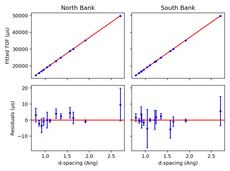
11. Check that in your save location there is a Calibration folder containing three .prm files ENGINX_305738 with the suffixes _all_banks, _bank_1, _bank_2.

12. Close the Engineering Diffraction gui and reopen it. The Load Existing Calibration radio button should be checked on the Calibration tab and the path should be populated with the _all_banks.prm file generated earlier in this test.

13. In the Load Existing Calibration box browse to the _bank_2.prm file and click the Load button.

Focus

1. Change to the Focus tab.

2. For the Sample Run # use 305761 and for the Vanadium # enter 307521.

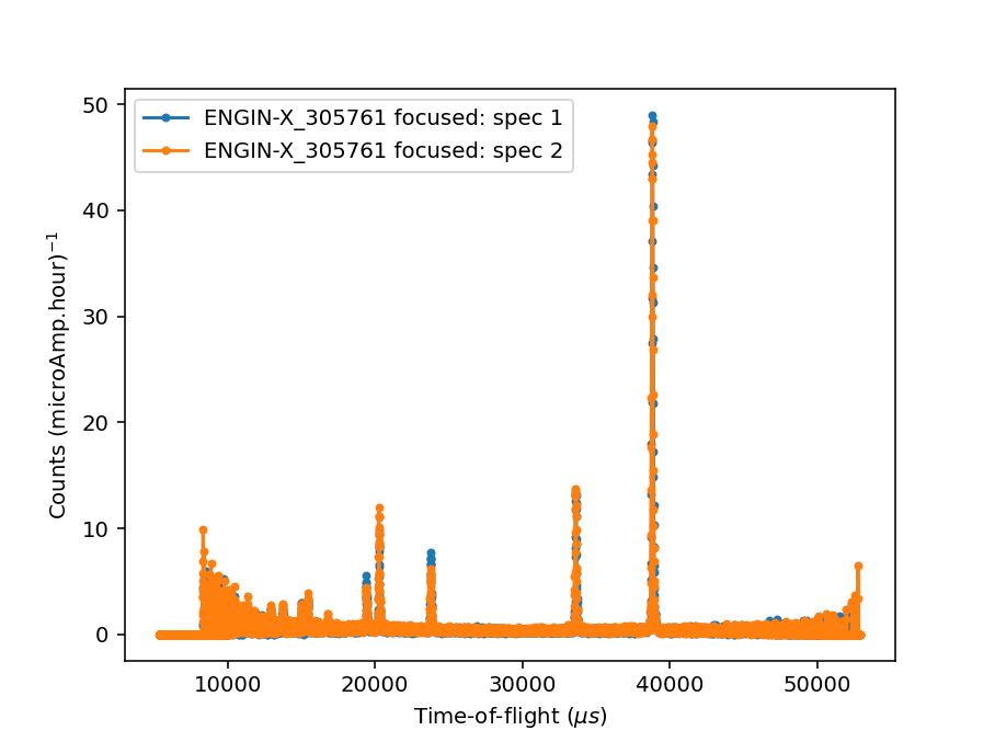
3. Tick the Plot Focused Workspace option and click Focus. It should produce a plot of a single spectrum for bank 2.

4. Go back to the Calibration tab and load in an existing calibration for both banks e.g. ENGINX_305738_all_banks.prm

5. Go back to the Focus tab and click Focus, after completing calibration it should produce a plot.

6. Check that in your save location there is a Focus folder containing the following files:

   • ENGINX_305738_305721_all_banks_dSpacing.abc

   • ENGINX_305738_305721_all_banks_dSpacing.gss

   • ENGINX_305738_305721_all_banks_TOF.abc

   • ENGINX_305738_305721_all_banks_TOF.gss

   • ENGINX_305738_305721_bank_1_dSpacing.nxs

   • ENGINX_305738_305721_bank_1_TOF.nxs

   • ENGINX_305738_305721_bank_2_dSpacing.abc

   • ENGINX_305738_305721_bank_2_dSpacing.gss

   • ENGINX_305738_305721_bank_2_dSpacing.nxs

   • ENGINX_305738_305721_bank_2_TOF.abc

   • ENGINX_305738_305721_bank_2_TOF.gss

   • ENGINX_305738_305721_bank_2_TOF.nxs

7. There should also be a CombinedFiles folder which should contain:

   • ENGINX_305761_307521_bank_dSpacing.nxs

   • ENGINX_305761_307521_bank_2_dSpacing.nxs

Test 2

This test covers the RB number.

1. Enter a string into the RB Number box.

2. Follow the steps of Test 1, any output files (for non-texture ROI) should now be located in both [Save location]/User/[RB number] and [Save location] (for texture ROI the files will be saved in the first location if an RB number is specified, otherwise they will be saved in the latter - this is to reduce the number of files being written).

Test 3

This test covers the Cropping functionality in the Calibration tab.

1. Change the RB Number to North, this is purely to separate the cropped output files into their own space.

2. Go to the Calibration tab, select Create New Calibration and tick the Set Calibration Region of Interest option. In the drop down Region of Interest select 1 (North).

3. Check the Plot Calibrated Workspace checkbox and click Calibrate.

4. The generated figure should show a plot of TOF vs d-spacing and plot showing residuals of the quadratic fit.

5. Check that only one .prm and one .nxs output file was generated.

6. Go to Focus tab and click Focus.

7. Change the RB number to Custom.

8. Set the Region Of Interest to Crop to Spectra and using Custom Spectra 1200-2400 (these spectrum numbers correspond to the South Bank). Please note that some custom spectra values may cause the algorithms to fail. Click Calibrate and a similar plot to before should appear but with only 2 subplots.

9. Set the Region of Interest to Texture (20 spec) and click Calibrate - there should be 20 spectra per run (5 tiled plot windows, 4 spectra per window).

Test 4

This test covers the sample setting functionality in the Absorption Correction tab.

1. Change the RB Number to ManualTesting.

2. Go to the Absorption Correction tab, in Sample Run(s) enter 305738 and click Load Files

3. A row should have been added to the table with Run: ENGINX00305738, Shape: Not Set, Material: Not set, and Orientation: default

4. Click Create Reference Workspace, ManualTesting_reference_workspace should now be listed as Reference Frame

5. In the Sample Shape section click Load Shape onto single WS

6. Make sure InputWorkspace and OutputWorkspace are set to ManualTesting_reference_workspace

7. Set Filename to a suitable file (<mantidBuildDir>/ExternalData/Testing/Data/UnitTest/cube.stl) and Scale to mm

8. There should now be a View button next to Shape in the Reference Workspace Information

9. Click this View button

10. If you have used the example STL you should get the following:

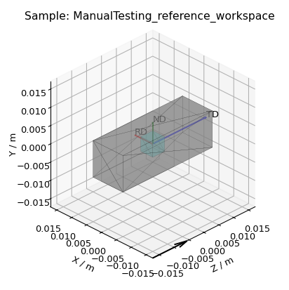
11. Now click Set Shape onto single WS and set InputWorkspace again to ManualTesting_reference_workspace

12. Set ShapeXML to:

..testcode:

<cuboid id='some-cuboid'> \
<height val='0.015'  /> \
<width val='0.012' />  \
<depth  val='0.012' />  \
<centre x='0.0' y='0.0' z='0.0'  />  \
</cuboid>  \
<algebra val='some-cuboid' /> \

13. Click Set Sample Material, set InputWorkspace to ManualTesting_reference_workspace and ChemicalFormula to Fe and click Run

14. Click Set Single Orientation and set the Workspace as ENGINX00305738 and set Axis0 to 90,1,0,0,1 and Axis1 to 135,0,0,1,-1, then click Run

15. Click either the checkbox in the table or Select All beneath the table to select the workspace and click Copy Reference Sample

16. The table should now be updated to Run: ENGINX00305738, Shape: [View Shape], Material: Fe, and Orientation: set

17. Open the settings menu (gear icon, bottom left)

18. Set Texture Directions to be D1  0  1  0, D2  1  0  0, and D3  0  0  1 and click OK

19. Down under the Include Absorption Correction change 4mmCube to Custom Shape

20. A new Custom Gauge Volume File field should have appeared, click Browse and navigate to <mantidBuildDir>/ExternalData/Testing/Data/SystemTest/Texture/custom_gauge_volume.xml

21. Clicking View Shape again, the shape should now look like:

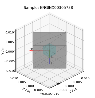
22. Click Apply Correction at the bottom of the tab

23. In the save directories, you should see an AbsorptionCorrection folder with Corrected_ENGINX00305738.nxs

24. Play around with other functionality (tool tips or Technique reference might be helpful) in this tab some things you can try:

• Load a collection of runs using the search 305793-305795

• Load runs from browsing (some more ENGINX data can be found in ExternalData/Testing/Data/SystemTest)

• Load Orientation File (some orientation files can be found in ExternalData/Testing/Data/SystemTest/Texture)

Test 5

This test covers the loading and plotting focused data in the fitting tab.

Note

Sometimes it will be tricky to load ENGINX files from the archive and the red * next to the Browse button won’t disappear. Proceeding with the red * will raise an error saying Check run numbers/path is valid. or Mantid is searching for data files. Please wait. In such cases, please try re-entering the text and wait till the red * is cleared before proceeding. If the log level is set to Information, found path = 1 will be visible in the message log when the runs are found from the archive.

1. Ensure you can access the ISIS data archive. In the Calibration tab, select Create New Calibration and enter Calibration sample # 305738. Before proceeding, make sure the red * next to the Browse button is disappeared when clicked somewhere outside that text box. Untick Set Calibration Region of Interest option and click on Calibrate button.

2. On the Focus tab, set Sample Run # to 305793-305795 and Vanadium # to 307521. These sample runs have different stress and strain log values. Make sure the red * s next to the two Browse buttons are cleared when clicked outside the text boxes or wait otherwise. Then click Focus.

3. In the Fitting tab, load multiple of these newly focused TOF .nxs files in the Load Focused Data section. The path to the focused files should be auto populated.

4. Click the Load button. A row should be added to the UI table for each focused run. There should be a grouped workspace with the suffix _logs_Fitting in the ADS with tables corresponding to each log value specified in the settings (to open the settings use the cog in the bottom left corner of the UI). In the same grouped workspace there should be an additional table called run_info_Fitting that provides some of the metadata for each run. Each row in these tables should correspond to the equivalent row in the UI table.

5. The log values that are averaged can be selected in the settings (cog button in the bottom left corner of the UI). Change which sample log checkboxes are selected. Close settings and then close and re-open the Engineering Diffraction interface. Reopen settings to check these selected sample logs have been remembered. Note that any change to the selected logs won’t take effect until the interface is reopened.

6. Clear the runs by clicking Remove All below the table. Repeat steps 1-2 above but this time try checking the Add To Plot checkbox, when loading the run(s) the data should now be plotted and the checkbox in the Plot column of the UI table should be checked.

7. Clear the runs by clicking Remove All below the table. Repeat steps 1-2 again but load the d-spacing .nxs file(s) instead.

8. Plot some data and un-dock the plot in the UI by dragging or double-clicking the bar at the top of the plot labelled Fit Plot. The plot can now be re-sized.

9. To dock it double click the Fit Plot bar (or drag to the bottom of the toolbar). You may want to un-dock it again for subsequent tests.

Test 6

This tests the Browse Filters functionality to filter the focused data in the Load Focused Data section at the top of Fitting tab.

1. The tests so far have enabled you to produce many different focussed data files. In the Load Focused Data section at the top of Fitting tab, when clicked on Browse button, check that the Unit Filter and Region Filter combo boxes help you to find dSpacing data for Texture regions and TOF data for North bank.

Test 7

This tests the removal of focused runs from the Fitting tab.

1. Load multiple runs using the Browse button. This should take you to a folder called “Focus” containing .nxs files that have been previously generated from the Focus tab. Select multiple files and click on Open

2. Having loaded multiple runs, select a row in the UI table and then click the Remove Selected button below the table. The row should be removed, if the run was plotted it will disappear from the plot and there should be one less row in each of the table workspaces inside the “_logs” workspace group with each row corresponding to the run in the same row of the UI table. The workspaces called “ENGINX_…._TOF” and “ENGINX_…._TOG_bgsub” will be deleted from the ADS

3. Try clicking the Remove All button, the UI table should be empty and the workspace group with name ending “_logs” should no longer be present.

4. Try loading in a run again, the UI should still be able to access the workspace and remember the log values - check there are no calls to AverageLogData in the log (should be visible when log level is Notice).

5. Try removing a workspace by deleting it in the ADS, the corresponding row in the log tables and the UI table should have been removed.

6. Delete a _bgsub workspace in the ADS, the corresponding row will not be deleted, but the Subtract BG checkbox will be unchecked.

Test 8

This tests that the background subtraction works.

1. Load in a run - the Subtract BG box should be checked in the UI table by default. This should generate a workspace with suffix _bgsub and the data should look like the background is flat and roughly zero on the plot using the default parameters (other columns in the UI table).

2. Select the row in the table and check the Inspect Background button should now be enabled regardless of whether the Subtract BG box is checked.

3. Click Inspect Background to open a new figure which shows the raw data, the background and the subtracted data. Changing the values of Niter, BG, XWindow and SG (input to EnggEstimateFocussedBackground, hover over a cell in the table to see a tool tip for explanation) should produce a change in the background on the external plot and in the UI plot.

Test 9

This tests the operation of the fit browser.

1. Check that when no data are plotted the Fit button on the toolbar does nothing.

2. Check the Unit Filter combobox for Browse Filters is set to TOF and click Browse. In the Focus folder of the save directory, there should be output focussed TOF files. Select multiple focussed files and click Open. Back on the main interface, check the box Add to Plot and click Load.

3. Click the Fit button in the plot toolbar. A simplified version of the standard mantid fit property browser should now be visible.

4. In the fit property browser, all the plotted spectra should be available in the Settings > Workspace combo box. In the central Run Selection table, remove one spectrum from the plot by unticking the Plot checkbox for one row. The Settings > Workspace combo box should now update and not include the removed spectrum.

5. Right-click on the plot image and select Add Peak and add a peak to the plot. Change the peak type by right clicking on the plot and selecting Select peak type and add another peak. Also add a Linear background by right clicking on the plot to select Add background and selecting LinearBackground as the function. Make sure to add a BackToBackExponential peak if you have not already. For BackToBackExponential peaks, the A and B parameters should be fixed automatically for ENGIN-X data.

6. Perform a fit by clicking Fit > Fit in the fit browser. On completion of the fit, a group workspace with suffix _fits should have appeared in the Workspaces Toolbox(ADS). In this group of workspaces there should be a matrix workspace for each parameter fitted (named by convention FunctionName_ParameterName e.g BackToBackExponential_I), to view this right-click on the workspace and Show Data. If there are more than 1 fitting function of the same type, the fitting values for each parameter would appear in the columns where each workspace is listed in the rows. Any runs not fit will have a NaN value in the Y and E fields. In addition there is a workspace that has converted any peak centres from TOF to d-spacing (suffix _dSpacing). There should be an additional table called model that summarises the chisq value and the function string including the best-fit parameters.

7. In the Fit property browser, go to Setup > Custom Setup. The function string, including the best-fit parameters, should also have been automatically saved as a custom setup. Select Setup > Clear Model, then select this new custom setup model. Inspect the fit by clicking Fit > Evaluate Function.

Test 10

This tests the sequential fitting capability of the UI (where the result of a fit to one workspace is used as the initial guess for the next). This test uses data generated in Test 4.

0. In the main workbench window, right-click on the Message log and set the Log Level to Notice.

1. Close and re-open the Engineering Diffraction interface.

2. Enter the Engineering Diffraction settings menu by clicking the cog wheel in the bottom left. In the Sample Logs - Fitting / GSAS II section, you can select which sample logs to output to table workspaces by ticking in the list of boxes, and select the Primary Log from the combo box underneath the checkboxes for Sequential fit ordering, and whether this should be in Ascending or Descending order by ticking the corresponding box to the right. In the Primary Log combobox, select ADC1_0 and tick Ascending.

3. On the Fitting tab, Load in several focused runs e.g. 305793-305795 from Test 4.

4. Plot just one run, click Fit to open the fit property browser and input a valid fit function including a peak and a background.

5. Click the Sequential Fit button in the plot toolbar. A group of fit workspaces should appear in the Workspaces Toolbox (ADS), each with a row for each of the runs in the table. All the runs should have been fitted.

6. The order of the runs in the sequential fit should be obtainable from the log at notice level - check that this corresponds to the order of the average value of the primary log - ADC1_0 You can check the value of this sample log for each run in the output GroupWorkspace with the suffix _logs_Fitting. Note this order down.

7. Try changing the primary log to blank and re-run the Sequential Fit This should make the Sequential fit use the order of the runs in the central Run Selection table.

8. In the Engineering Diffraction settings, set the Primary Log back to ADC1_0 and tick Descending. Re-run the Sequential Fit and check that the order of runs in the output workspaces has reversed compared to Step 6.

9. Close and re-open the Engineering Diffraction interface. Reopen the Engineering Diffraction settings menu, it should remember the Primary Log and the order.

Test 11

This tests the serial fitting capability of the UI (where all loaded workspaces are fitted from the same starting parameters). This test uses data generated in Test 4.

1. Repeat steps 1-4 in the previous test (Test 9).

2. Now click the Serial Fit button in the plot toolbar and the group of fit workspaces should appear in the ADS, each with a row for each of the runs in the table. All the runs should have been fitted.

3. The order of the runs in the serial fit should be obtainable from the log at notice level - check that this corresponds to the order of the runs in the table.

Test 12

This test will check the Pole Figure plotting in the Texture Tab

1. Click on the Texture Tab

2. Click Browse next to Load Workspace Files and navigate to <mantidBuildDir>/ExternalData/Testing/Data/SystemTest/Texture/ValidationFiles/Focus

3. Select all the files within that folder and click Load Workspace Files

4. You should see seven rows populate the table

5. Click on any of the View Sample buttons and verify it displays the sample and the sample axes + labels

6. Click Select All Files

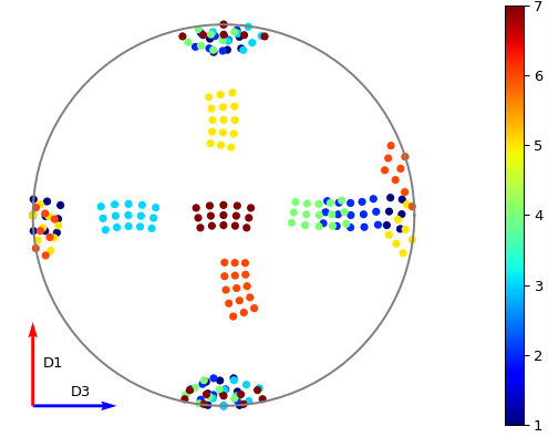
7. In settings, ensure the texture directions are set to D1  1  0  0, D2  0  1  0, and D3  0  0  1, and the Scatter Plot Experimental Pole Figure is checked, then click OK

8. Click Calculate Pole Figure, you should get a plot like the one below

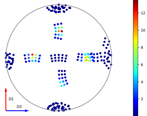
9. Now click Browse next to Load Parameter Files and navigate to <mantidBuildDir>/ExternalData/Testing/Data/SystemTest/Texture/ValidationFiles/FitParameters

10. Select all the files within that folder and click Load Parameter Files

11. The Fit Parameters column should now be populated in the table, as well as a readout column option having appeared above Calculate Pole Figure

12. Click Calculate Pole Figure, you should get a plot like the one below

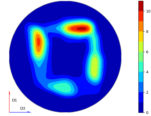
13. Open the settings menu and set Scatter Plot Experimental Pole Figure to unchecked

14. This should enable Contour Kernel Size, set this to 6.0 and click OK

15. Click Calculate Pole Figure, you should get a plot like the one below

16. Try changing options around in the interface, see if you can break it (some things you can try if you are short ideas):

• Try different sample axes

• Try changing the projection

• Try including scattering power (HKL for this peak is 1,1,0 if you set the crystal to the Fe.cif)

• Try disabling some of the rows

• Try having a mixture of runs with/without parameter files

Test 13

Note this test will only work if GSASII is also installed. Please test this on IDAaaS: an ENGINX instance should have MantidWorkbenchNightly and GSASII installed in the expected location.

1. Close and re-open the Engineering Diffraction interface.

2. Go to the Calibration tab, select Create New Calibration and un-tick the Set Calibration Region of Interest option.

3. For the Calibration Sample # enter 305738 and click the Calibrate button.

4. On the Focus tab, enter Sample Run # 305761 and Vanadium # 307521 and click the Focus button.

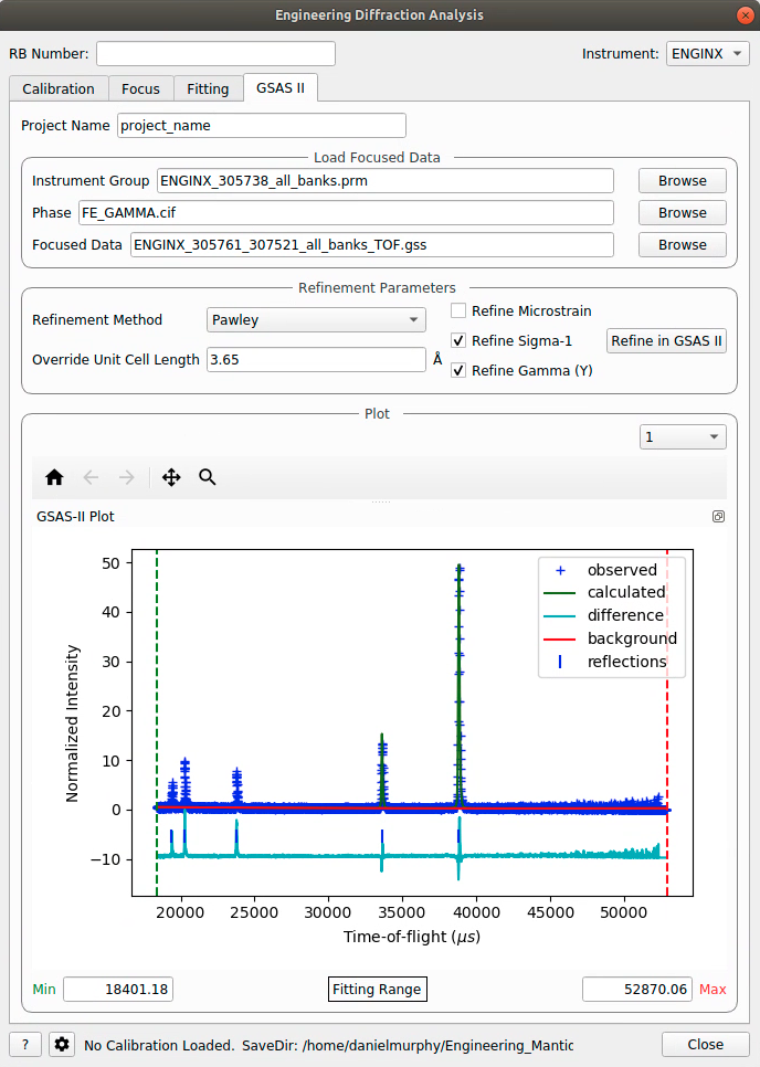
5. Change to the GSASII tab. The Instrument Group path should be pre-filled to a .prm file output by the calibration and the Focused Data path should be pre-filled to the .gss file output from the Focus tab.

6. For the Phase filepath, browse to MANTID_INSTALL_DIRECTORY/scripts/Engineering/ENGINX/phase_info/FE_GAMMA.cif. For the Project Name at the top, enter a string of your choice.

7. Now, click Refine in GSAS II. After a few seconds, the output fit should be plotted. In the top right of the plot widget, the refined spectrum can be changed using the combo-box.

8. Change the fitting range by dragging the limits, or by editing the Min, Max line edit boxes. Again, click Refine in GSAS II and this should only fit to the user defined range.

9. Back in the file loading section, Browse for files for the inputs Instrument Group and Focused Data, and select files with bank_1 in the name, which were produced by the Calibration and Focus in Test 3.

10. Now, click Refine in GSAS II. The previously set fitting range should be ignored as new input files were selected. There should now only be one spectrum available in the output spectrum combobox.

11. Set the Override Unit Cell Length to 3.65 and click Refine in GSAS II, the fit should be better.

12. Tick all the checkboxes: Microstrain, Sigma-1 and Gamma (Y). An asterisk should appear with an advice tooltip.

Test 12

This test covers the multiple data files functionality with multiple banks per file in the GSASII tab.

Note this test will only work if GSASII is also installed. Please test this on IDAaaS: an ENGINX instance should have MantidWorkbenchNightly and GSASII installed in the expected location.

1. Close and re-open the Engineering Diffraction interface.

2. Go to the Calibration tab, select Create New Calibration and un-tick the Set Calibration Region of Interest option.

3. For the Calibration Sample # enter 305738 and click the Calibrate button.

4. On the Focus tab, enter Sample Run # 305793-305795 and Vanadium # 307521 and click the Focus button. This will generate multiple focused data files. Change to the GSASII tab. Clear any pre-filled paths.

5. For the Instrument Group filepath, browse and select the single .prm file output by the calibration (should be ENGINX_305738_all_banks.prm).

6. For the Focused Data filepath, browse and select multiple .gss files that each contain multiple banks. Ensure all selected files have the same number of banks (e.g., select the all_banks files: ENGINX_305738_305793_all_banks_dSpacing.gss, ENGINX_305738_305794_all_banks_dSpacing.gss, ENGINX_305738_305795_all_banks_dSpacing.gss).

7. For the Phase filepath, browse to MANTID_INSTALL_DIRECTORY/scripts/Engineering/ENGINX/phase_info/FE_GAMMA.cif. For the Project Name at the top, enter a string of your choice.

8. Click Refine in GSAS II. After a few seconds, the output fit should be plotted. In the top right of the plot widget, verify that the refined spectrum combobox shows entries for the banks of the last refined data file.

9. Test Error Cases: Try selecting multiple instrument .prm files (should show error message about requiring exactly one instrument file). Try selecting .gss files with different numbers of banks (should show error about inconsistent bank counts). Try selecting single-bank .gss files (should show error about requiring multiple banks per file).