Muon Unscripted Testing: HIFI#
Introduction#
These tests looks at data from the HIFI instrument. The first test will introduce dead time corrections. When a detector receives a signal, there is small period of time afterwards when it can not record a new signal. This is called the dead time. We can model and adjust the data to compensate for the dead time. When looking at the raw counts, which look like an exponential decay, the correction makes the biggest difference at large count values. The second test will use multiple periods, this is when the same data is recorded twice at slightly different time intervals.
HIFI Transverse Field Simultaneous Fitting#
Time required 5 - 10 minutes
Open Muon Analysis (Interfaces > Muon > Muon Analysis)
Change Instrument to HIFI, found in the Home tab
In the loading bar enter
134028-39Some new data will appear in the plot
- Go to the grouping tab
In the group table, tick the
Analyseoption forfwdIn the pair table below, untick the
Analyseoption forlong
- Go to the Corrections tab
Set the plot to
Counts(combobox above the plot), you will now see an exponential decayChange the dead time correction to
Noneand notice that the counts at small times decreasesChange the dead time correction back to
From Data File
- Go to the Grouping tab
In the Pair table, click Guess Alpha
In the resulting dialog, change the run to
HIFI134034to be used for the calculationA value close to
1.3should appear
- Go to the Fitting tab
Check the Simultaneous fit over checkbox, and change from Run to Group/Pair
Right click the empty table area; Select Add Function
Add a FlatBackground (Background > Flat Background)
Similarly, add ExpDecayOsc (Muon > MuonGeneric > ExpDecOsc)
Set all parameters to Global, except Frequency
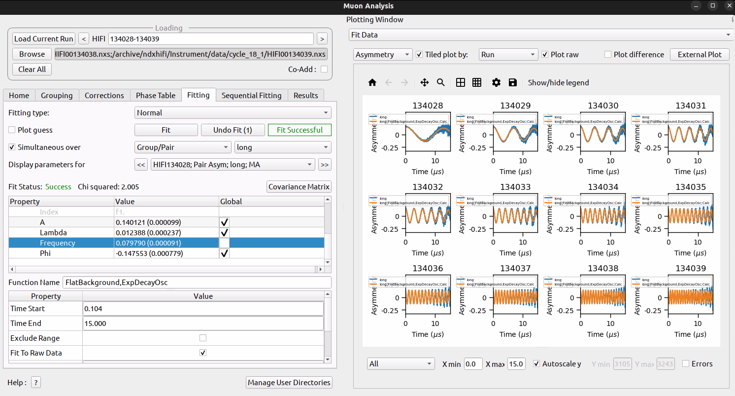
Click Fit
The fit might work but with a large Chi-squared Squared value (
>100)- Now to try the fit a different way.
Click Undo Fits
Click the value for the Frequency parameter; A
...should appear next to it, click it. A new window should appearEnter a value of
0.01for the first run in the tableFor each of the other runs in the table, enter values from
0.1to1.1in steps of0.1Click Ok
Click Fit
This time the fit should work with a significantly lower value for Chi-squared (
<10)
Tick
Tiled plot byin the plotting windowChange the combobox to
Runand each subplot will now contain just 2 linesCheck that the lines look similar to the results below
HIFI MultiPeriod Data#
Time required 5 - 10 minutes
In the loading bar enter
84447-9Go to the Grouping tab and press
Default- Go to the Fitting tab
Untick
Tiled plot byin the plotting windowUntick
Simultaneous over
- Go to the Sequential Fitting tab
Press
Sequentially fit allWhen its complete the table should update
It is ok if some of the rows say “Failed”. This happens because these rows need more iterations to converge. However, if you go to the Fitting tab and cycle through the datasets, you can see that the fits are still reasonably good.
Selecting rows will show you the data and fit for those rows
- Go to the Grouping tab
The
Periodcolumn in the group table will show a series of numbers (1, 2, 3 or 4)Press the
Periodsbutton and a pop up will appear with 5 rows (one spare)Close the pop up
Tick the
Analysebox in the grouping table for “fwd1”Untick all of the
Analyseboxes in the pair tableThis will leave you with 3 lines (one for each run)
In the
Periodscolumn you can sum periods by using a comma seperated list or a range using a dashWhen you change the periods summed the plot will change